April 7, 2017 anaylsis politics
This is the second post in a two-part series, examining presidential election results from Pennsylvania. If you haven’t read Part 1 yet, you should start there.
In my first post, we examined election data from 2016 (and some from 2012) and uncovered some interesting results on what Trump did right. Nevertheless, many people (myself included and, arguably, a majority of the US population) were surprised by the election results. At this point I became curious: should we have been surprised? Was this apparent sweep truly unprecedented? After all, we heard a lot about how this was the first year in a long time that Pennsylvania “went red”, but how did this year actually stack up against previous elections?
To shed some light on these questions, we can take a more comprehensive look at data from previous elections. So, I gathered county-level results for every presidential election in Pennsylvania since 19961, and registration data since 2000. In this post, we re-examine several of the metrics discussed in Part 1 for previous elections, to see if there are larger trends that have been at play in Pennsylvania elections.
Historical Election Results
We start with a look at the voting results from all elections since 1996.
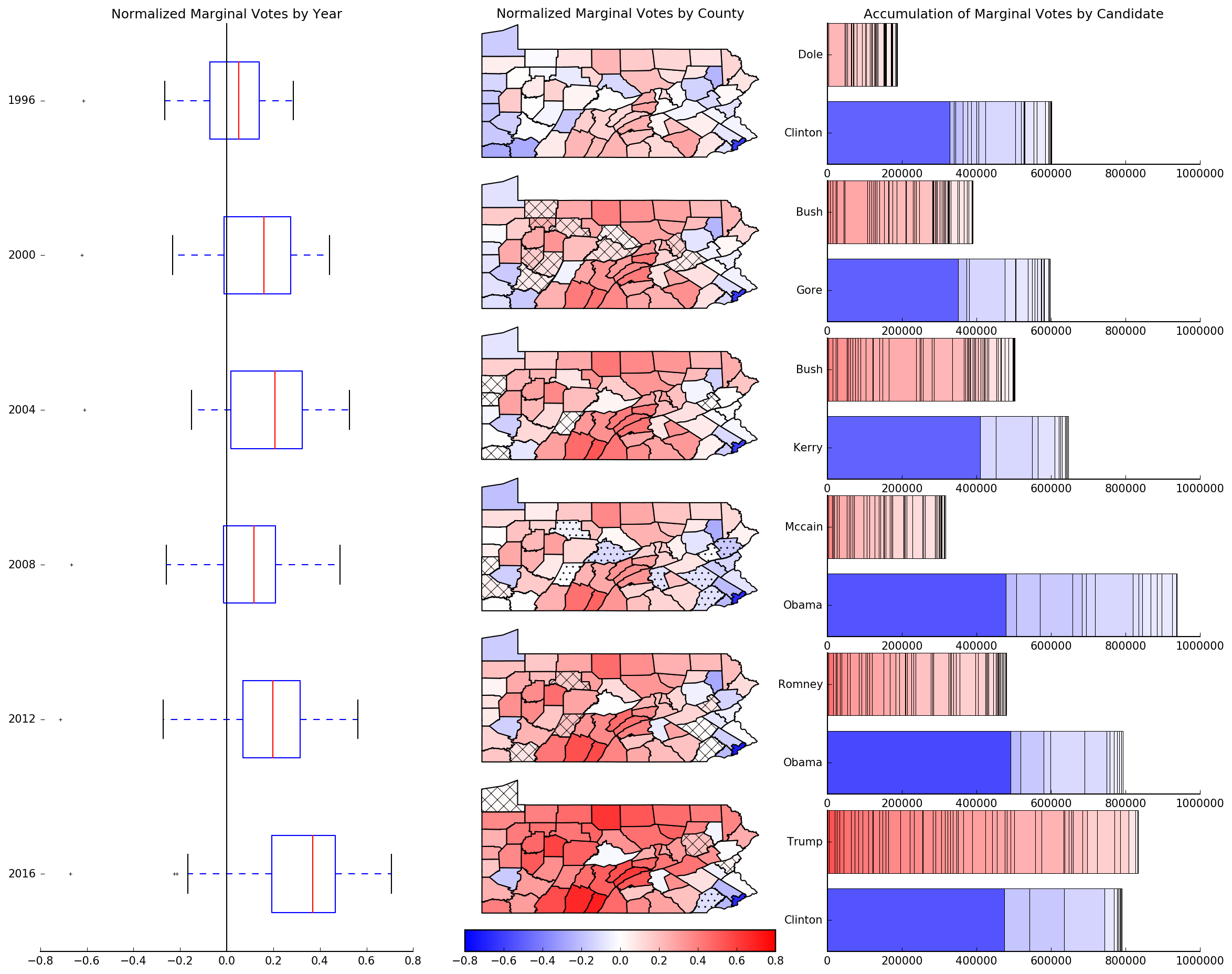
Fig 1. Three different ways of visualizing the normalized marginal votes by county from elections 1996-2016: Tukey boxplots (left), on a map (center) and as stacked bar charts, by candidate (right). The boxplots and map show the normalized marginal votes (as a percentage), while the bar charts show total marginal votes.
While it’s tempting to see Trump’s victory as an anomaly (the “first time in recent history Pennsylvania has gone red” perspective), Figure 1 tells a more nuanced story. Indeed, the first thing you should notice is the gradual yet steady shift across the state towards the right since the 1996 election. From this perspective, 2008 appears to be the anomaly. It’s the only election when the distribution of marginal votes actually shifted slightly back to the left. To achieve this, Obama won an extraordinary number of additional marginal votes while McCain lost around 100,000. Every other year, we see the number of marginal votes for Republicans steadily rising while Democrats maintain. In 2016, Trump managed to make two elections’ worth of gains in one, and how he did that was the focus of the first part of this series.
This trend to the right is reinforced by examining flipped counties. With the exception of Chester county in 2016, 2008 is the only year since 1996 when any county flipped Democrat. That means that since 1996, a net of 17 counties have flipped from voting Democrat (in 1996) to Republican (in 2016).
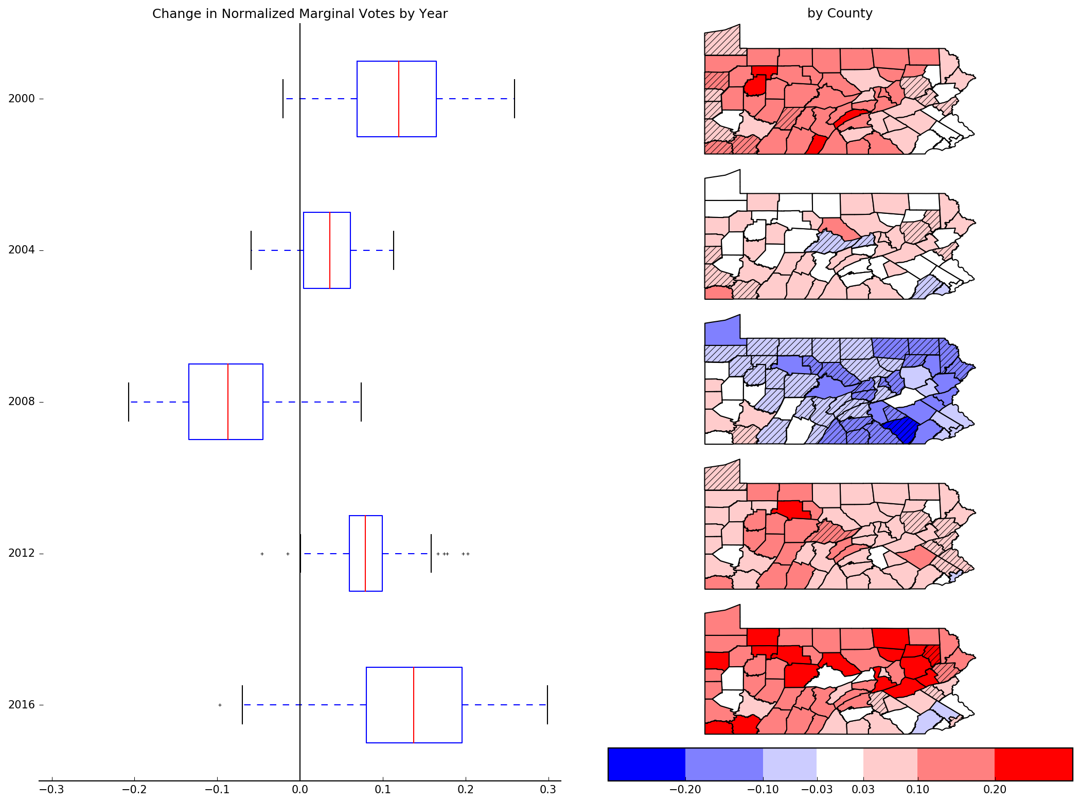
Fig 2. Visualizing changes in normalized marginal votes for years 1996-2016 with: Tukey boxplots (left) and on a map (right). In each map, every county is colored according to its shift in normalized marginal votes from the previous year. Counties in which votes shifted away from the winning candidate have been shaded.
I provide Figure 2 simply because it is the clearest way of seeing how widespread the shift to the right has been in the state, even amongst counties which continue voting Democrat. Also, I found it surprising how most of the counties exhibit shifts of >3% every year, and most often in the same direction for each election.
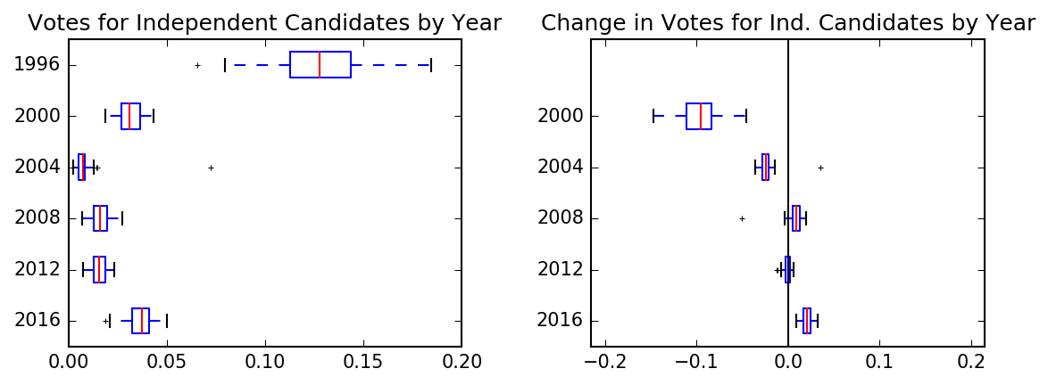
Fig 3. Plotting percentage of votes for independent candidates (left) and its difference (right) from the elections in 1996-2016.
Finally, we wrap up this section by looking at how the independent vote has changed over the years in Figure 3. Although votes for independent candidates rose in 2016, it was comparable to 2000 and is totally dwarfed by 1996. Further, while votes for independent candidates increased in every county in 2016, this shift is insignificant in scale when compared with the shift in normalized marginal votes (seen in Figure 2). Taken together, these two facts suggest that the number of votes garnered by independent candidates this year was normal and consistent with previous elections.
Historical Registration Data
Looking at results is one thing, but as we saw in Part 1, looking at registration data can also be insightful. To start, let’s look at how the basic registration variables have changed over the years2.

Fig 4. Distributions by year of (from left to right): total registered voters, relative registered Republicans, and turnout. The second row shows how each variable changed between elections. Registered voters is normalized by the county population estimates for each year.
From Figure 4, note that the total number of registered voters has remained somewhat stable in Pennsylvania since 2000. It rose by less than 10% in most counties since 2000, and actually declined in many 2012.
Unsurprisingly, 2016 saw the highest turnout of the past 5 elections. However, I’m surprised to see that turnout dropped in 2008 - it seemed with how many extra MV Obama won, it would have been due at least in part to higher turnout. Further indication of how anomalous 2008 really was.
Finally, if we compare Figure 4 with Figure 2, it seems that the change in relative Republican registrations has varied similarly to the change in normalized marginal votes for each election. But the shifts in relative Republican registrations are much less pronounced. Let’s see just how the two variables correlate.

Fig 5. Plots change in relative Republican registrations against change in normalized marginal votes for each county in each election. Points are colored according to the party of the winning in that county in that election (red=Republicans, blue=Democrats).
As Figure 5 indicates, the variables are indeed positively correlated, matching our intuition above. I find it interesting how the 2008 and 2016 distributions are distributed over a wider range, while 2004 and 2012 are much more condensed around the origin. It’s also remarkable how few counties exhibit opposing shifts (shift positive in registrations but negative in votes, or vice versa). While this is typical of correlated variables, I’m still surprised by how few counties fall in the second or fourth quadrants of the plots.
Also, as we noted above, the shift in votes is generally of a higher magnitude than the shift in registrations. I guess both are somewhat intuitive, but together they suggest that we might be able to assemble a primitive estimator for election results by looking at how registrations shifted since the previous election. But I leave that for future exploration.
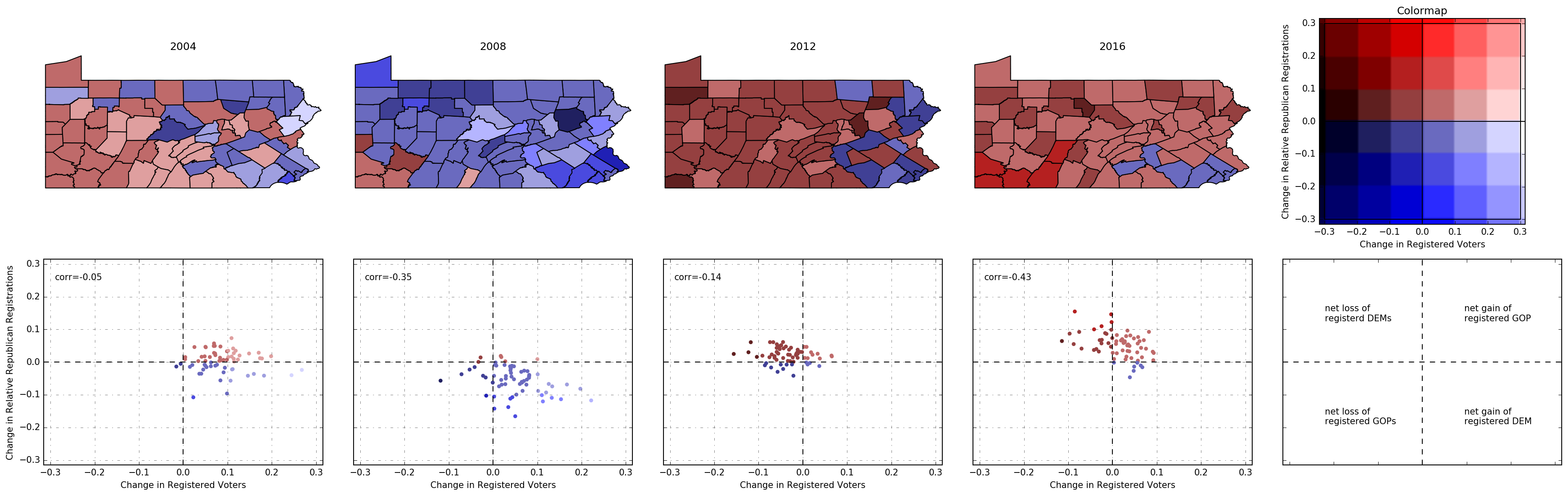
Fig 6. Visualizing how the changes in registered voters and relative Republican registrations between elections are distributed geographically (top) and along the two axes (bottom).
Finally, I wanted to explore how changes in total registrations and relative Republican registrations jointly varied, because I was curious if there was any relation between the two (perhaps as a result of voter suppression/purging, etc.) In Figure 6, each point plotted in the bottom row corresponds to a county from the map above, and every county is colored according to the discretized 2D colormap on the right. The legend in the bottom right gives a general way of interpreting the plots based on which quadrant each county is in. For example, counties in the upper left quadrant experienced a net loss of registrations but a shift towards a larger percentage of voters registered Republican, meaning that there must have been a net loss of registered Democrats.
One thing that’s apparent from the figure is that the shifts are not strongly correlated across the state. However, it is interesting that the southwestern counties are the only ones to consistently see increases in relative percentage of Republicans registered, while the southeastern counties have only gotten more Democrat-leaning in registrations.
Summary of all Data, by County

Fig 7. Visualizing a subset of the examined variables for the counties home to the 5 largest cities in Pennsylvania.
Figure 7 presents the statistics for the counties where the 5 largest cities in Pennsylvania (Philadelphia, Pittsburgh, Allentown, Erie, and Reading) reside. Nothing in particular jumps out at me, I just find it an interesting visualization. It doesn’t fit nicely on a single page, but I’ve also generated the same plots for every county here.
A very obvious curiosity is if one can train a classifier on this data to see if we can cluster the counties. I made some feeble attempts but didn’t find any meaningful clusters.
Closing Thoughts
In the wake of the 2016 election we heard, in the media and on social media, many exceptional stories about how all the polls were wrong and how surprising the result was to many people. From that, many of us, myself included, extrapolated that this election was anomalous - that something crazy happened that’s never happened before. And while that may have been true about the state of the political climate in the US or the rhetoric of the campaigns, the data doesn’t support that conclusion. If anything, 2008 was the anomaly in recent elections. As Part 1 concluded, Trump did many things to win, but that win was just a hastening of an existing trend towards voting for Republican candidates in Pennsylvania.
Producing this second post was challenging because going back in time provided a whole variety of exciting ways to analyze the data. Every time I’d sit down to answer one question, I’d wind up with 5 more questions to investigate next. Choosing which parts of my analysis to pull out and clean up for this post was a challenge, to say the least. As a result, the post is a bit more like a collection of interesting figures than a cohesive narrative building to a singular conclusion. Nevertheless, I hope you enjoyed it.
As I mentioned at the end of Part 1, all data and code for generating the results and figures in this series, plus a lot of code and figures which didn’t make it into the posts, is available on Github. Someday, I’d like to come back and continue this exploration, but if you’re excited about it, please jump in and let me know what you find!
Edit: After I wrote most of this post, I discovered Data for Democracy had released county-level election and registration data from the 2016 election for most states. And they are supposedly working on gathering historical data as well. So it may be a lot easier to run this analysis on other states in the future!
Thanks to Karen Hao, Ryan Ko, Andrew Zukoski, Shane Leese and Lakshman Sankar for reading drafts of this.
Why 1996? Somewhat arbitrary, although it gives us context from the last two party shifts in the presidency (Bush in ‘00 and Obama in ‘08). Also, the Pennsylvania state website only hosts results since 2000, so I had to get creative in my google searches. Finally, I hope one day to run this analysis for other states, and the farther I go back, the more data I’d need to format and parse to analyze other states (where I can even get it at all). Call me lazy.
↩As mentioned before, 1996 is missing when we consider registration data because I couldn’t find it at the county level.
↩